Fundamentals of Algorithms
Table of Contents
1 Algorithm - the basics
- algorithm is a finite steps of instructions to solve a problem
- Algorithms normally represented in one of the three ways:
- psuedo-code
- flowchart
- structured English
- Algorithms can be assessed based on time complexity and space complexity
- Time complexity is the measure of how much time an algorithm needed
- Space complexity is the measure of how much space an algorithm needed
2 Recursive Algorithms
Recursive Algorithm Basics
- Recursive algorithms have the following characteristics:
- A recursive algorithm must have a base case to allow it to terminate/return.
- A recursive algorithm must change its state and move toward the base case.
- A recursive algorithm must call itself, recursively.
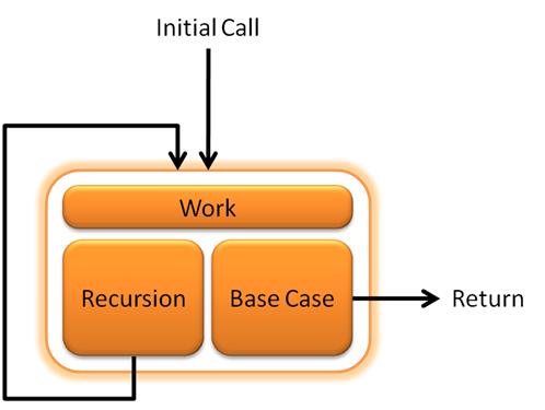
- recursive algorithms are for solving problems of recursive nature
- An example of a recursive problem is the factorial calculation of an integer N, for example 4!= 4 x 3 x 2 x 1
- the base case is when the number is 1, 1!=1. (0! = 1 as well!)
- the recursion lies in the fact that N! = N x (N-1)! = N x (N-1) X (N-2)! so on and so further
- A Python implementation of this algorithm in recursion is:
# Recusiion for factorial
# AKA n*(n-1)*(n-2) until n-m = 1

def factorial(n):

    if n == 1:
	return 1
    else:
	# recursive call to itself with successively smaller
	# argument to the function towards the base case
	return n*factorial(n-1)

# calling the function to test
print(factorial(5))
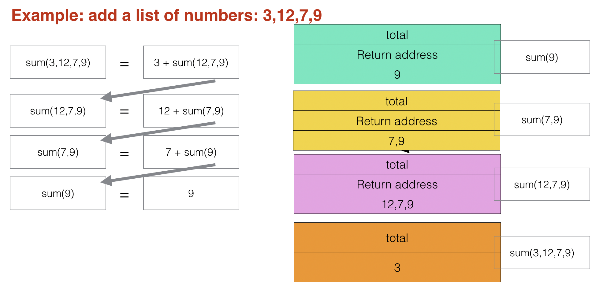
- Another example of a recursive problem is to add a sequence of number
- the base case is when the number of items to add is 1
- the recursion lies in the fact that sum(N1 + N2 + .. + Nm) = N1 + sum(N2 + N3 + N4
…Nm) = N1 + N2 + sum(N3N4 +…Nm) so on and so further - A Python implementation of this algorithm in recursion is:
def listsum(numList):

   # the base case where only one item in the list
   if len(numList) == 1:
	return numList[0]
   else:
	return numList[0] + listsum(numList[1:])

print(listsum([1,3,5,7,9]))
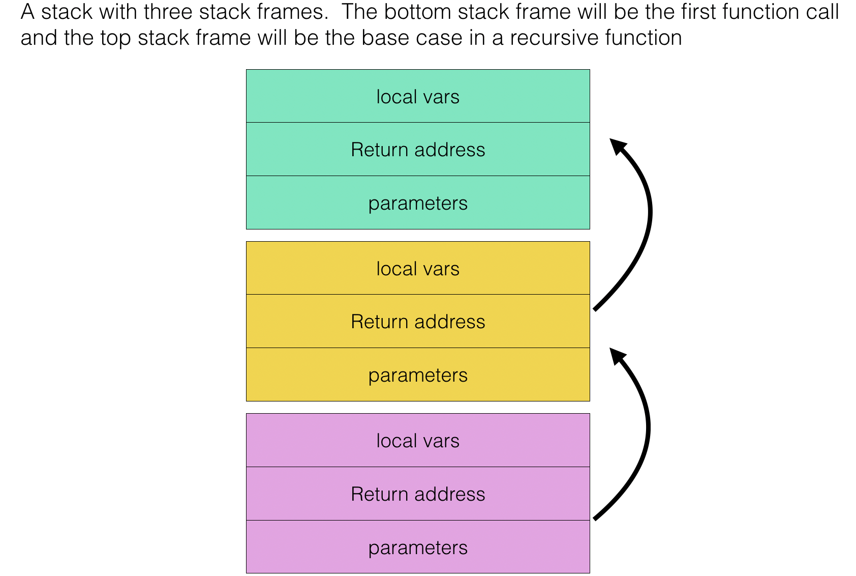
Recursive Algorithm and Call Stack
A call stackis composed ofstack frame. As the name implies it is of stack data structure- Each stack frame corresponds to a call to a subroutine that has not yet terminated, with each frame:
- holding return address of function
- holding parameters
- holding local variables
- Stack has limited size
overflow: pushing to an already full stackunderflow: pop from an empty stack
- A recursive function may contain several calls to itself.
- each call, a return address is being pushed onto the stack
- when recursion ends, the return address is popped one after another, thus ends the call.
- if a mistake is made during recursion, and it never ends, the stack will eventually overflow and the program crashes.
- Take the recursive algorithm of the sum of a list of numbers above, when the first time that function listsum called, a stack frame is created and pushed onto the call stack.
- As the next recursive call made with the rest of list, except the first item, another stack frame is created and pushed onto the call stack.
- The above steps repeats until the base case reached and the final function call stack frame popped from the stack and return to its caller which is the stack frame just underneath it.
3 The Big-O notation
- Big-O notation is a way of measure the time complexity of algorithms
- As time requirement is closely related to number of operations, this is normally measured in the number of operations, thus the O in Big-O
- It is important to understand that Big-O notation is a measure on how the time will grow as the number of data input grow.
- Big-O provides the worst case measure for time
- You are expected to:
- know the five Big-O functions
- calculate time complexity and express it in Big-O notation for a given algorithm
- rank time complexity functions in the order of their efficiency
Constant Time Function - O(1)
- This notation means an algorithm has the time complexity of a constant - regardless of the growth of data input size, the algorithm will take the same amount of time.
- An example: access an item in a dictionary (hashtable) will take the same time regardless how big the dictionary is. Another example will be when checking if a number is even or odd by using the modular operation.
Logarithmic Time Function - O(logN)(assuming log base 2 in this note)
- Just to re-cap some basic logarithmic operations:
- log28 = 3
- log216 = 4
- log232 = 5
- This notation means an algorithm will increase its time by 1 when its input size doubled.
- An example: binary search. As shown in the following figure, even the array size has doubled(right hand side), there is only one more comparison added.
Linear Time Function - O(N)
- This notation means an algorithm has the time complexity of a linear function - as the data input size grows, the algorithm will take the amount of time that is directly proportionate to the input size.
- An example: linear search (remember Big-O is for the worst case) as the number of items increases, so is the number of comparisons.
Polynomial Time Function - O(N2)
- This notation means as the data input size increases, the time required will be squared.
- An example: bubble sort where as the number of items increases, the worst case number of operations will be square of the number of items.
Exponential Time Function - O(2N)
- This notation means for every added input item, the time required will be doubled.
- This time complexity is for intractable problems which are problems cannot be solved using polynomial time or less. The algorithms for this type problems are not optimal for computers to run in a reasonable amount time to be useful.
- An example: the travelling salesman problem(TSP) where a salesman has to visit N towns. Each pair of towns is joined by a route of a given length. Find the shortest possible route that visits all the towns and returns to the starting point. The time increases exponentially for large N.
Time Complexity Comparision
- From most time eficient to least:
- O(1)
- O(logN)
- O(N)
- O(N2)
- O(2N)
4 Searching algorithms
Linear Search
- linear search is a simple algorithm that seek a value in a collection
- In English, the algorithm works as following:
- Starting from the first item in a list
- Comparing the search value with the item
- If equal, return found
- Else, move to the next item
- Repeating step 2 to step 4 until either the end of the list or return found
- The algorithm can be expressed in pseudo-code as following:
FUNCTION LinearSearch(myArray, searchValue)
    found = False
    FOR item in myArray
        IF item == searchValue
           found = True
        ENDIF
    ENDFOR
    RETURN found
END
- Can you work out the time complexity of linear search?
- Aim to implement this algorithm with a given list of items and user input for the searchValue with data validation for user input
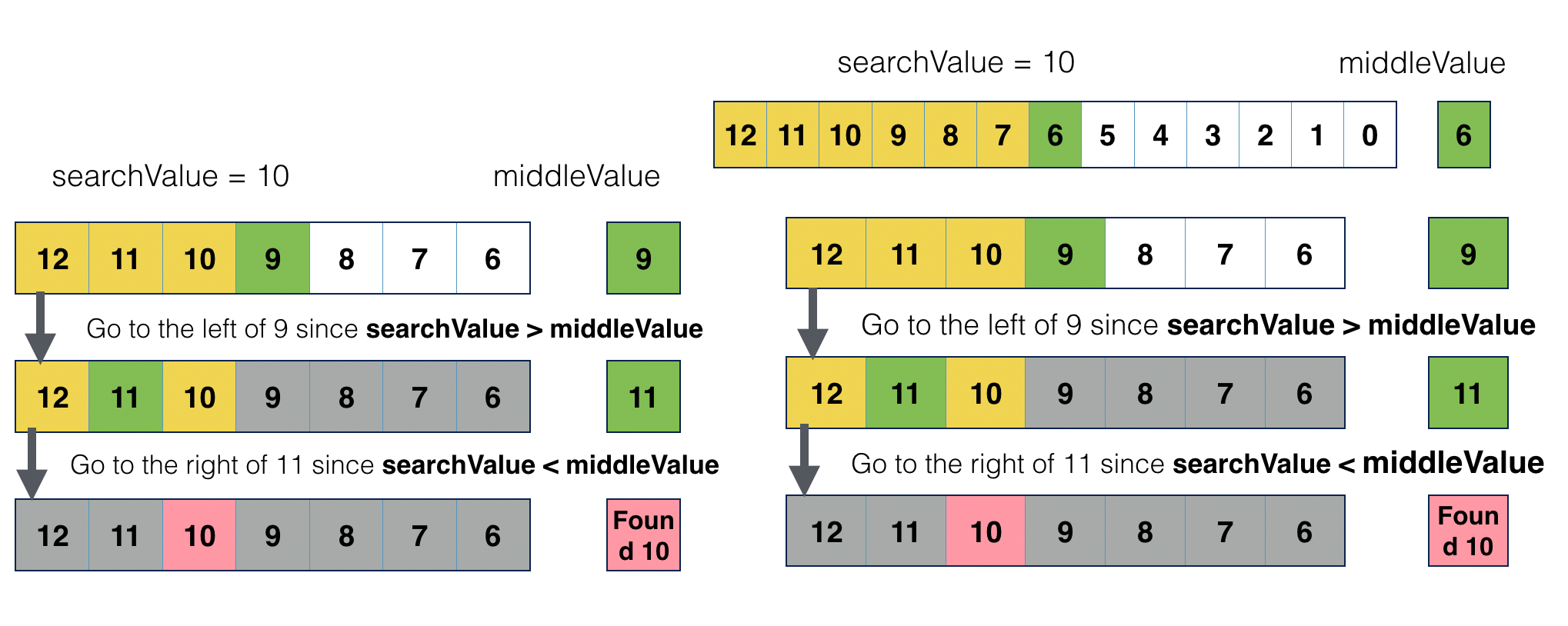
Binary Search
- Binary search works with a sorted list of items
- It compares the search value with the middle item,
- if the middle item equals the search value, found
- if the search value is greater than the middle value, perform the same search method in the list of items that are greater than the middle item
- if the search value is smaller than the middle value, perform the same search method in the list of items that are smaller than the middle item
.
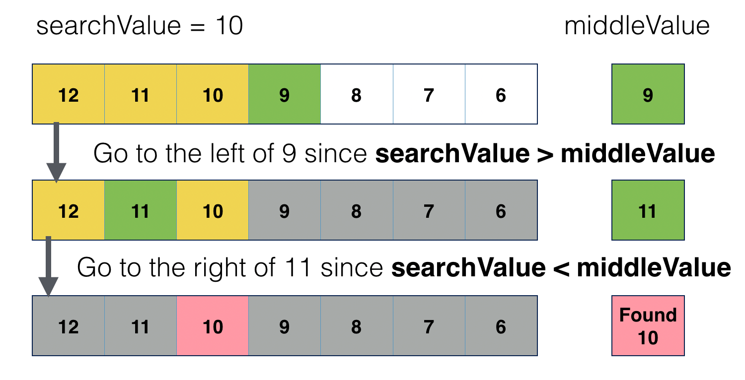
- the pseudo-code for binary search can be expressed as following:
- Try to work out the time complexity for binary search (hint: see note on Big-O)
FUNCTION BinarySearch(myArray, searchValue)
     low = 0
     high = len(myArray)-1
     WHILE low <= high
         mid = (low + high) / 2
         IF myArray[mid] > searchValue
             high = mid - 1
         ELES IF myArray[mid] < searchValue
             low = mid + 1
         ELSE
             RETURN mid
         ENDIF
     ENDWHILE

     RETURN "Not Found"
 END
- You may ask what if the number of items in the list is even? There will be no middle item.
- In this case, the algorithm will still work as long as the middle item is picked using a consistent method. It does not matter which side of the half has one more item.
- Aim to implement the above algorithm for various length array of various data types
- Later, you will see the same algorithm implemented in recursive.
Binary Tree Search
- Binary search works from a BST - Binary Search Tree (see data structure section)
- The algorithm works like this:
- Starting from the root node, comparing with its value
- Either skip the left or the right half of the subtree
- Repeat the process with the subtree, until found or not found
- In the later section on recursive algorithms, we will look at this search algorithm in more details.
- Aim to :
- implement a BTS using recursion
- calculate its complexity and express it in the Big-O notation
5 Sorting algorithms
Bubble sort
- Bubble sort is a classic sorting algorithm
- It is not very efficient, especially when there are many items in the collection.
- The algorithm works like this:
- Starting from the first item in a list/array, comparing with its value with the next item, swap if necessary.
- Move to the next item, repeat step 1 for the rest of items. This is called a pass
- After the first pass, the largest value will be moved to the end assuming sorting the list in ascending order
- Repeat the process again, “bubble” the next largest item to its correct place.
- Bubble sort pseudo-code:
FUNCTION bubbleSort(myArray):
    FOR i=0 TO len(myArray)-2
        FOR j=0 TO len(myArray)-2:
            IF myArray[i]>myArray[i+1]:
                temp = myArray[i]
                myArray[i] = myArray[i+1]
                myArray[i+1] = temp
            ENDIF
        ENDFOR
    ENDFOR
END
- There are two FOR loops for the algorithm. This means, if we have an array with 8 items, the total number of loops will be 8x8 = 64.
- Although you can reduce the total number of loops (can you work out how?) as the the number of items in their correct places increases, there are still two loops.
- Can you work out the time complexity for bubble sort?
Merge sort
- Merge sort is more efficient than Bubble sort. It works like this:
- Dividing the list into n sublist, each contains one item
- Repeatedly merge sublists to produce new sorted lists until there is only one sublist remaining.
- The list is sorted
- In recursive algorithm:
- if one element in the list, it is already sorted, return.
- divide the list recursively into two halves until it cannot be divided.
- merge the smaller lists(n number of lists) into new list in sorted order.
- A gif to help you visualise this:
- Can you work out the time complexity?
- The time complexity for merge sort is not as straight forward as the previous algorithms.
- It's O(N * log(N)), not O(log(N)), this is becuase the entire input will be halved O(log(N)) times, during the merge stage, each item must be iterated through. Therefore log(N)*N, gives O(Nlog(N)).
6 Traversal Algorithms
Simple Graph-travesal Algorithms - Depth First
- Depth first traversal(DFT), AKA as depth first search(DFS) works by visiting from a starting node, and visiting as many nodes as it can along each branch before backtracking.
- It is implemented using a stack.
- The stack is used to store a list of visited nodes along a branch and then popped as it backtracks to the starting node.
- The following is the pseudo-code for this algorithm:
G is a graph and V is the starting node
S is a stack data structure

FUNCTION DFS(G,v)
    Initiliase Stack S
    visited = []
    FOREACH node u in G
       visited[u] = false
    S.push(v)
    WHILE S is not empty
       u = s.pop()
       IF not visited[u]
          visited[u] = true
          FOREACH unvisited neighbour w of u
             S.push(w)
          ENDFOR
       ENFIF
    ENDWHILE
 END
- Here is a website with images to help you understand how DFS works
Simple Graph-travesal Algorithms - Breadth First
- Breadth first traversal(BFT), AKA as breadth first search(BFS) works by visiting from a starting node, and visiting the closest nodes first.
- It is implemented using a queue.
- The queue is used to store a list of unvisited nodes closest to the current node and then dequeue it as it visits each immediate node.
- Start by putting any one of the graph's vertices at the back of a queue.
- Take the front item of the queue and add it to the visited list.
- Create a list of that vertex's adjacent nodes. Add the ones which aren't in the visited list to the back of the queue.
- Keep repeating steps 2 and 3 until the queue is empty.
- The following is the pseudo-code for this algorithm:
FUNCTION BFS(G, v)
    Initialise Queue Q
    visited = []
    WHILE Q is not empty
        u = Q.dequeue()
        FOREACH neighbour of u
            visited[u] = false
            Q.enqueue(u)
        ENDFOR
    ENDWHILE
END
- Here is a website with images to help you.
Simple Tree-travesal Algorithms
- See Fundamentals of Data Structures-Tree for the three tree traversal
- Pseudo-code for the three traversals:
- In-Order traversal:
p is a node on a tree, it starts from the root node tree is a data structure Function inOrderTraverse(p): IF tree[p].left <> -1 inOrderTraverse(tree[p].left) EndIF Output tree[p].data IF tree[p].right <> -1 inOrderTraverse(tree[p].right) EndIF End Function - Post-Order traversal:
p is a node on a tree, it starts from the root node tree is a data structure Function inOrderTraverse(p): IF tree[p].left <> -1 inOrderTraverse(tree[p].left) EndIF IF tree[p].right <> -1 inOrderTraverse(tree[p].right) EndIF Output tree[p].data End Function - Pre-Order traversal:
p is a node on a tree, it starts from the root node
tree is a data structure

Function inOrderTraverse(p):

    Output tree[p].data

    IF tree[p].left <> -1
       inOrderTraverse(tree[p].left)
    EndIF

    IF tree[p].right <> -1
       inOrderTraverse(tree[p].right)
    EndIF

End Function
- In-Order traversal:
7 Reverse Polish, Infix and Prefix Notations
Infix notation - 9 * 6 + 12
- This notation is used in arithmetical and logical formulae and statements.
- In this notation, operators are placed between operands they operated on: 9 * 6 + 12
Prefix notation - + * 9 6 12
- Also known as normal Polish notation (NPN)
- It eliminates the need for brackets in expressions
- operators are placed before the operands they operate on: + * 9 6 12
Reverse Polish notation(RPN) - + * 9 6 12
- Also known as Postfix notation
- It eliminates the need for brackets in expressions
- operators are placed after the operands they operate on: 9 6 * 12 +
- You are expected to:
- underdstand the significance of Reverse Polish notation (RPN)
- convert from RPN to infix and from infix to RPN
- construct a expression tree from a RPN expression vice versa
- RPN used in programming languages for syntax due the following advantages:
- It does not need any parentheses as long as each operator has a fixed number of operands
- It is easier for computers to evaluate expressions using stacks
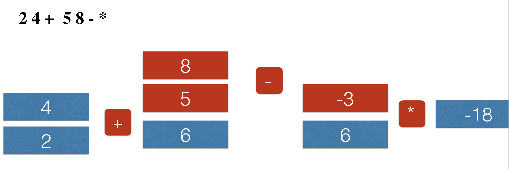
Convert from Infix to RPN
- example 1:
(2+4)*(5-8) —> 2 4 + 5 8 - *
- example 2:
infix:  (9-4) * (6+7) - (24/2 + 5)
RPN:  9 4 - 6 7 + * 24 2  / 5 + -
- example 3:
infix:  2 * 3 + 12/4
RPN:  2   3   *  12    4  /  +
- follow this link and finish the exercises on the page
Evaluate RPN using stack
- starting from the left most token of an expression
- push the operands onto the stack until an operator encounted
- pop two operands from the stack and apply the operator
- push the result from step 2 onto the stack
- repeat this process until end of the expression
- Example:
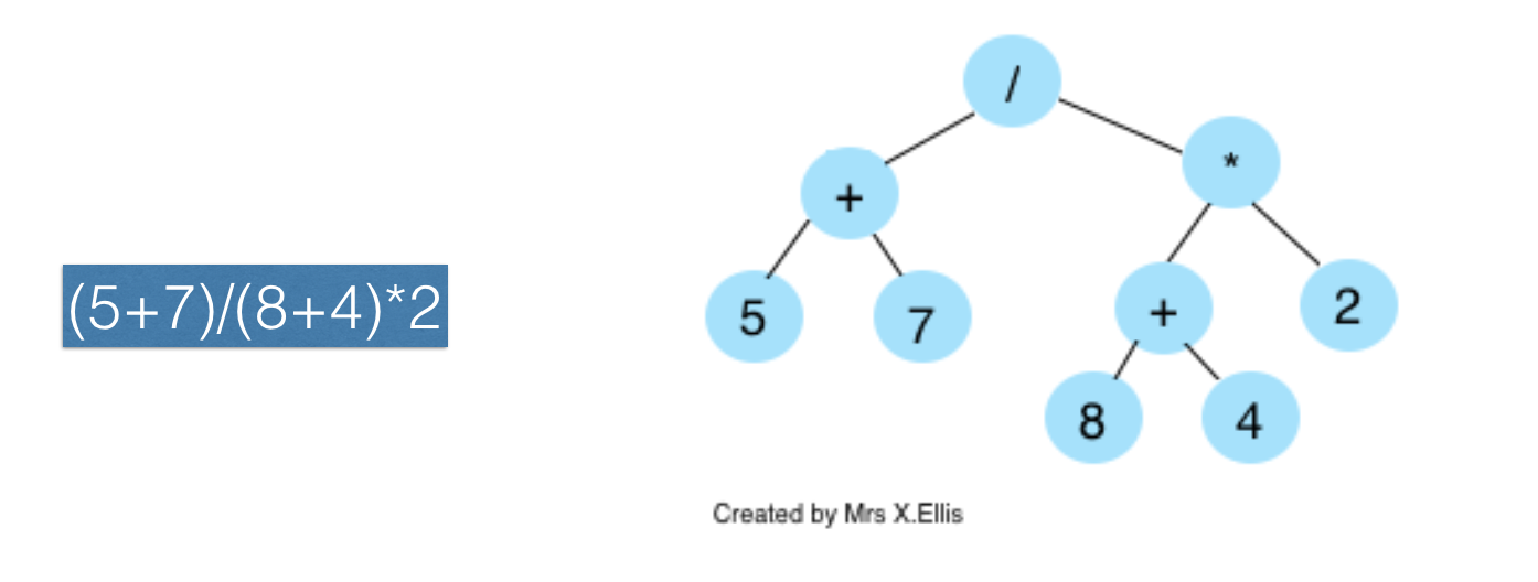
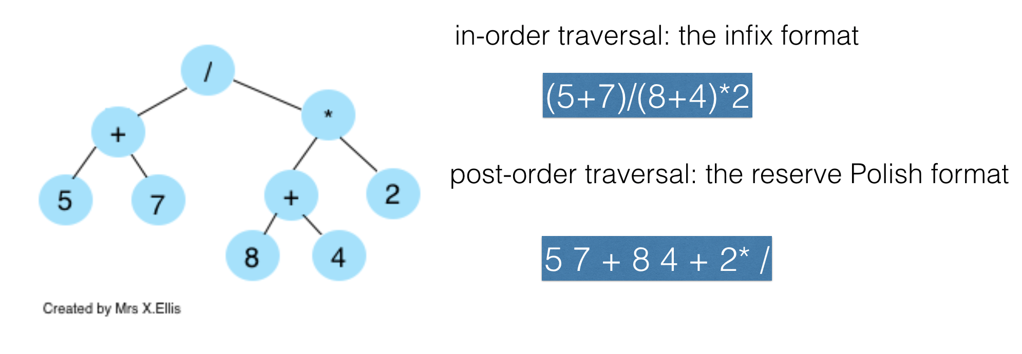
Building a RPN from an expression tree
- Consider this infix expression : (5+7)/(8+4)*2
- To build a binary expression tree, find an operator from proximately middle of the expression, in this case "/" as the root node
- on either side of this root node, we will left with two subtrees to build
- again, pick an operator in the middle of the left or right sub expression and add this as a child node to the root node
- all leaf nodes should be operands
- example:
Binary expression tree to infix, RPN
- Once a Binary Expression Tree exists, different tree traversal algorithms can produce infix, postfix (RPN) or prefix expression.
- To obtain RPN, just apply post-order tree traversal
- To obtain infix, just apply in-order tree traversal
8 Optimisation algorithms
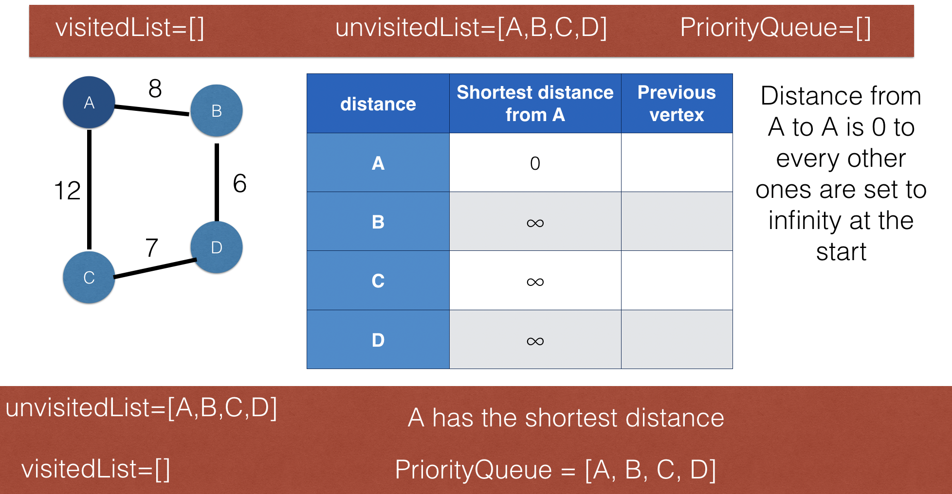
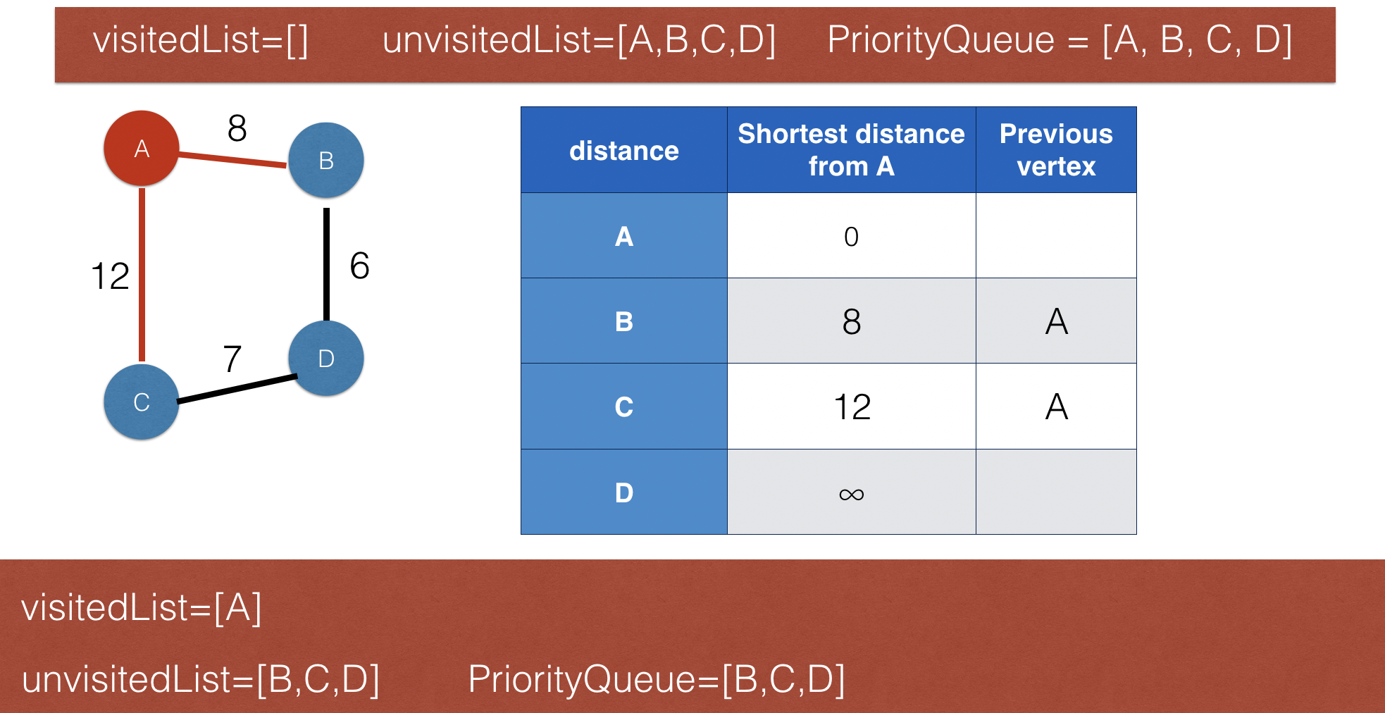
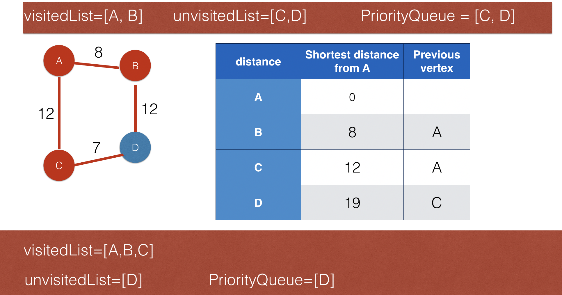
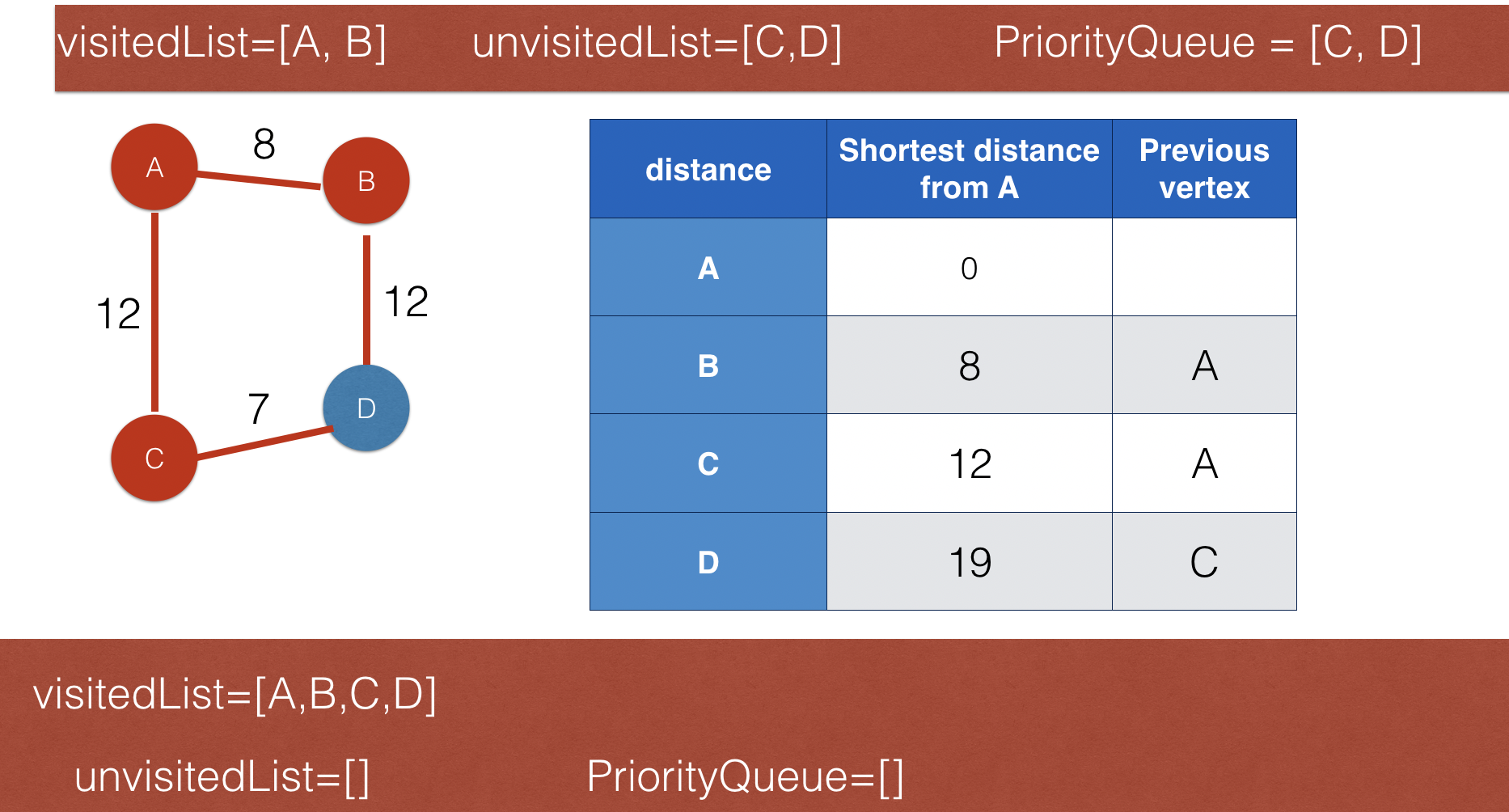
Dijkstra’s shortest path algorithm
- One if the well-known optimisation algorithms
- It's purpose is to find the shortest distance from a starting node to anany other nodea in a connected graph
- Dijkstra algorithms is implemented using a priority queue, and it is a variant of BFS.
- It keeps two lists: visited nodes kept in one and unvisited nodes in the other
- The following images using a simple graph to illustrate how this algorithm works. x

- Here is a video to help you if you are still unsure